Examples

Reading a LAZ file

import startinpy

dt = startinpy.DT()
dt.read_las("/home/elvis/myfile.laz", classification=[2,6])
print("# vertices:", dt.number_of_vertices())

Exporting the DT to GeoJSON

import startinpy
import numpy as np

#-- generate 100 points randomly in the plane
rng = np.random.default_rng(seed=42)
pts = rng.random((100, 3))
dt = startinpy.DT()
dt.insert(pts, insertionstrategy="AsIs")
dt.write_geojson("/home/elvis/myfile.geojson")

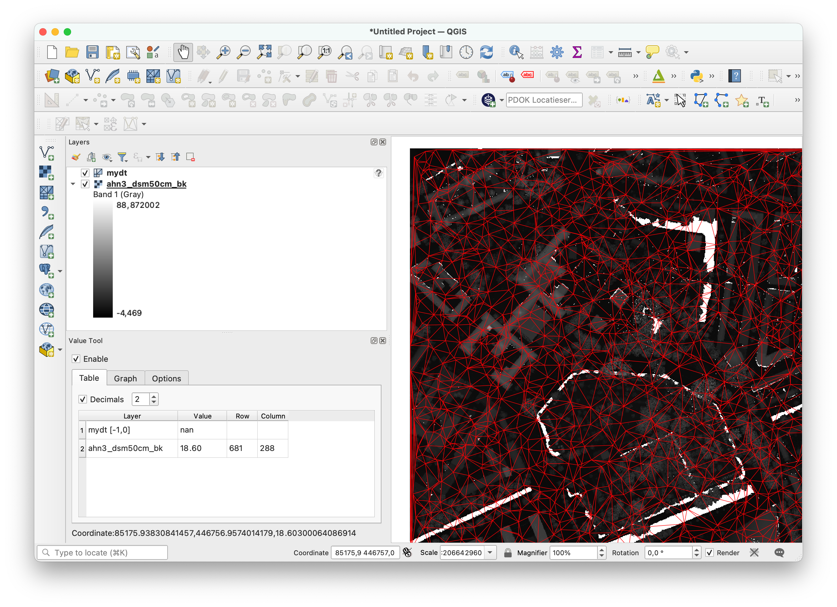
Reading a GeoTIFF file with rasterio

We can use rasterio to read a GeoTIFF and triangulate the centre of the pixels/cells directly. Notice that retrieving the (x,y)-coordinates of the centres with the xy() function of rasterio is super slow and it’s better to use the code below.

Notice that we use the insertion strategy “BBox” because it is several orders of magnitude faster for gridded datasets.

The no_data values are not inserted in the triangulation.

This code saves the resulting triangulation to a PLY file that can be opened directly in QGIS (with the newish MDAL mesh).

import startinpy
import rasterio

d = rasterio.open('mydem.tif')
band1 = d.read(1)
t = d.transform
pts = []
for i in range(band1.shape[0]):
    for j in range(band1.shape[1]):
         x = t[2] + (j * t[0]) + (t[0] / 2)
         y = t[5] + (i * t[4]) + (t[4] / 2)
         z = band1[i][j]
         if z != d.nodatavals:
             pts.append([x, y, z])
dt = startinpy.DT()
dt.insert(pts, insertionstrategy="BBox")
#-- exaggerate the elevation by a factor 2.0
dt.vertical_exaggeration(2.0)
dt.write_ply("mydt.ply")

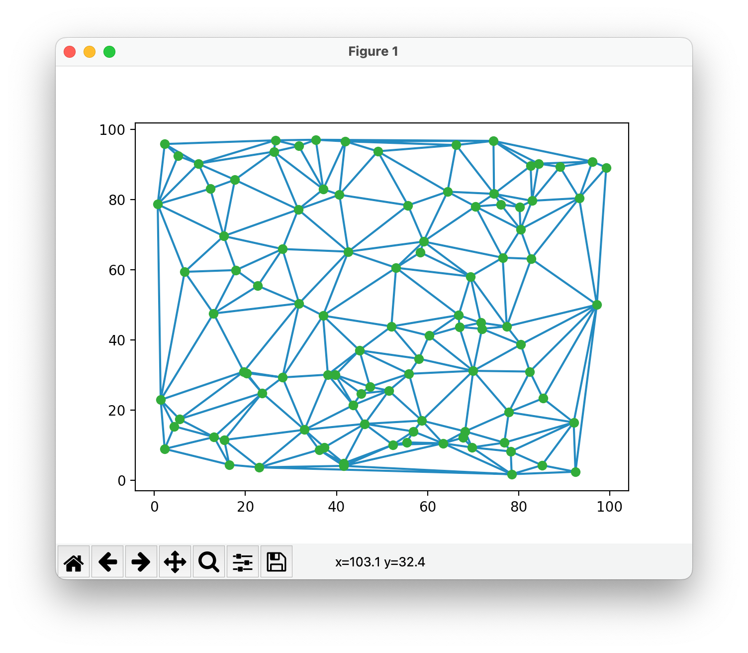
Plotting the DT with matplotlib

import startinpy
import numpy as np

#-- generate 100 points randomly in the plane
rng = np.random.default_rng(seed=42)
pts = rng.random((100, 3))
#-- scale to [0, 100]
pts = pts * 100
t = startinpy.DT()
t.insert(pts)
pts = t.points
trs = t.triangles
#-- plot
import matplotlib.pyplot as plt
plt.triplot(pts[:,0], pts[:,1], trs)
#-- the vertex "0" shouldn't be plotted, so start at 1
plt.plot(pts[1:,0], pts[1:,1], 'o')
plt.show()