Examples
Reading a LAZ file
We recommend you use laspy (pip install 'laspy[lazrs]' to install) to read a LAS/LAZ into a NumPy array, and then pass that array to startinpy:
import startinpy
import numpy as np
import laspy

las = laspy.read("myfile.laz")
pts = np.vstack((las.x, las.y, las.z)).transpose()
pts = pts[::1] #-- thinning to speed up, put ::10 to keep 1/10 of the points
dt = startinpy.DT()
dt.insert(pts)
print("number vertices:", dt.number_of_vertices())
Exporting the DT to GeoJSON
import startinpy
import numpy as np

#-- generate 100 points randomly in the plane
rng = np.random.default_rng(seed=42)
pts = rng.random((100, 3))
dt = startinpy.DT()
dt.insert(pts, insertionstrategy="AsIs")
dt.write_geojson("myfile.geojson")
Exporting the DT to several mesh formats with meshio
import startinpy
import meshio
import laspy
import numpy as np

las = laspy.read("../data/small.laz")
pts = np.vstack((las.x, las.y, las.z)).transpose()
dt = startinpy.DT()
dt.insert(pts)
vs = dt.points
vs[0] = vs[1] #-- to ensure that infinite vertex is not blocking the viz
cells = [("triangle", dt.triangles)]
meshio.write_points_cells("mydt.vtu", vs, cells)
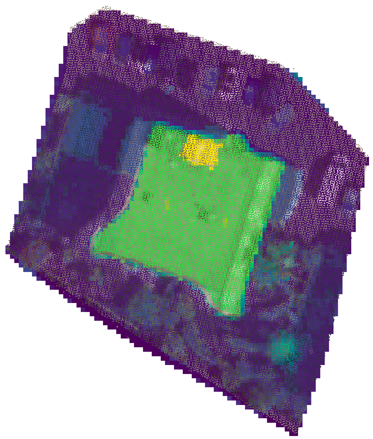
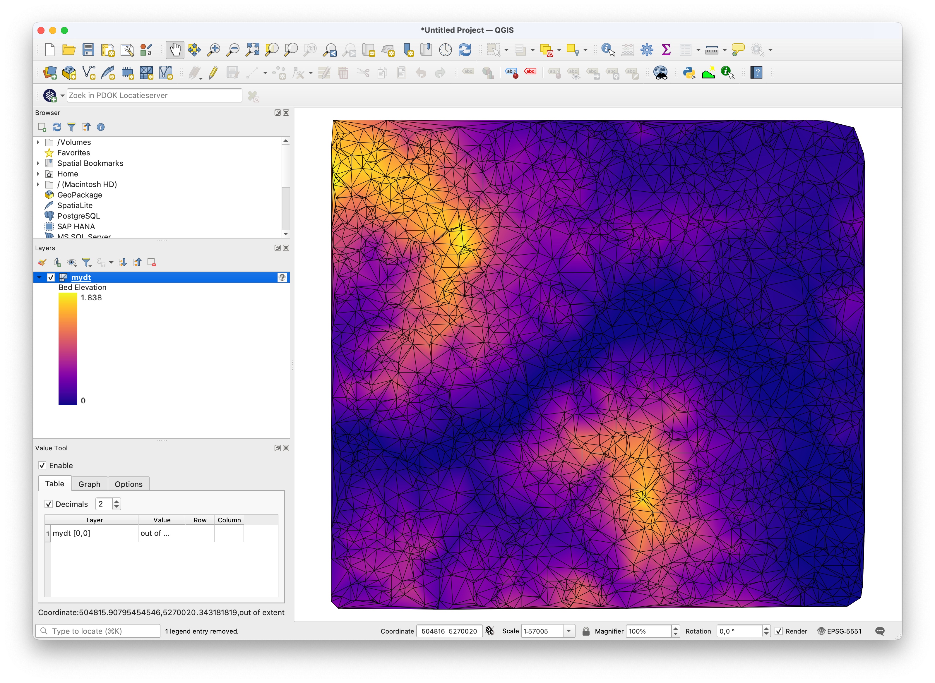
Reading a GeoTIFF file with rasterio
We can use rasterio to read a GeoTIFF and triangulate the centre of the pixels/cells directly. Notice that retrieving the (x,y)-coordinates of the centres with the xy() function of rasterio is super slow and it’s better to use the code below.
Notice that we use the insertion strategy “BBox” because it is several orders of magnitude faster for gridded datasets. The code also randomly selects 1% of the points.
The no_data values are not inserted in the triangulation.
This code saves the resulting triangulation to a PLY file that can be opened directly in QGIS (with the newish MDAL mesh).
import startinpy
import rasterio
import random

d = rasterio.open('../data/dem_01.tif')
band1 = d.read(1)
t = d.transform
pts = []
for i in range(band1.shape[0]):
    for j in range(band1.shape[1]):
         x = t[2] + (j * t[0]) + (t[0] / 2)
         y = t[5] + (i * t[4]) + (t[4] / 2)
         z = band1[i][j]
         #-- skip no_data + select randomly only 1% of the points
         if (z != d.nodatavals) and (random.randint(0, 100) == 5):
             pts.append([x, y, z])
dt = startinpy.DT()
dt.insert(pts, insertionstrategy="BBox")
#-- exaggerate the elevation by a factor 2.0
dt.vertical_exaggeration(2.0)
dt.write_ply("mydt.ply")
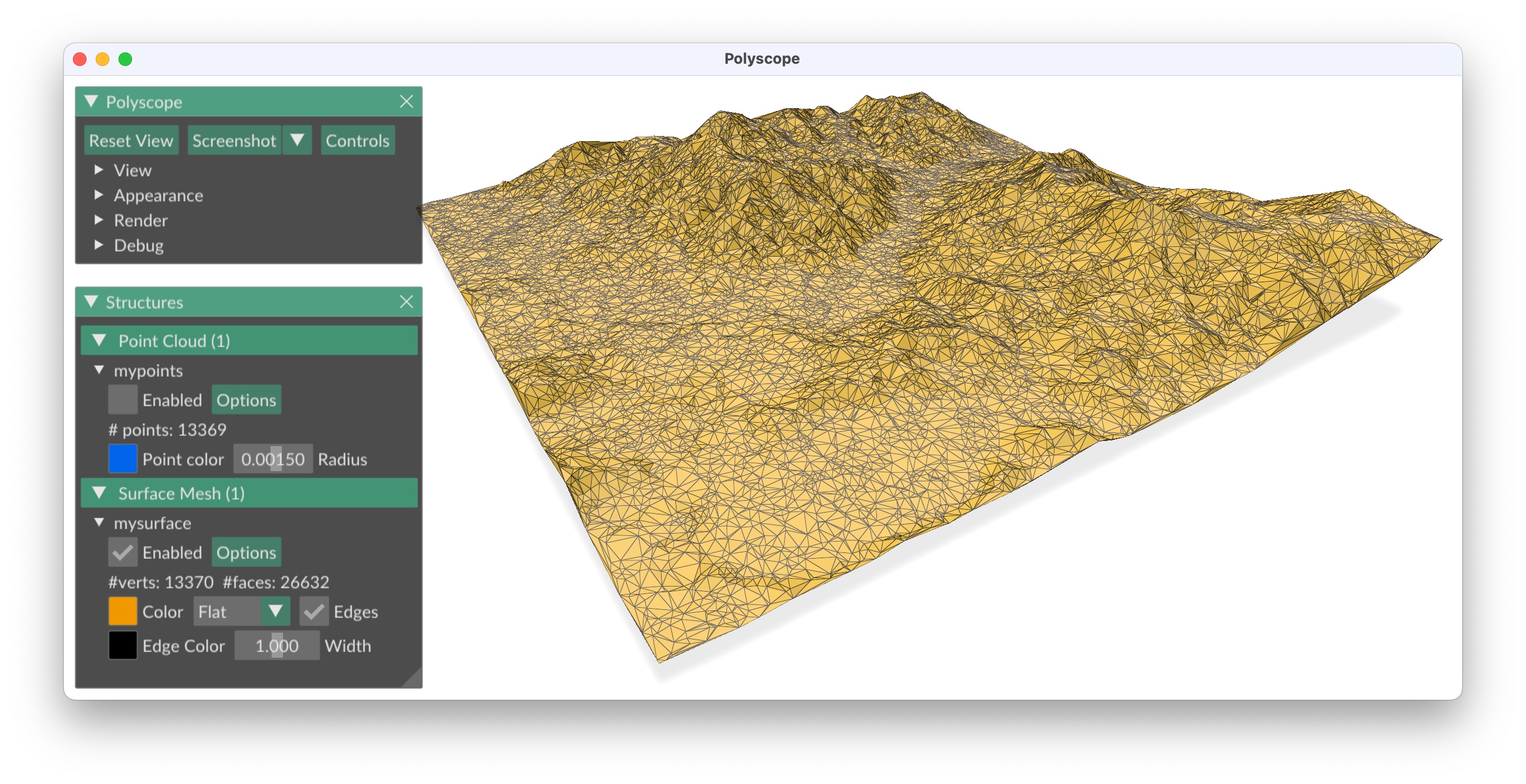
3D visualisation with Polyscope
You need to install Polyscope (basically pip install polyscope).
import startinpy
import numpy as np
import polyscope as ps
import laspy

las = laspy.read("data/small.laz")
pts = np.vstack((las.x, las.y, las.z)).transpose()
pts = pts[::10] #-- thinning to speed up, put ::10 to keep 1/10 of the points
dt = startinpy.DT()
dt.insert(pts)

pts = dt.points
pts[0] = pts[1] #-- first vertex has inf and could mess things
trs = dt.triangles

ps.init()
ps.set_program_name("mydt")
ps.set_up_dir("z_up")
ps.set_ground_plane_mode("shadow_only")
ps.set_ground_plane_height_factor(0.01, is_relative=True)
ps.set_autocenter_structures(True)
ps.set_autoscale_structures(True)
pc = ps.register_point_cloud("mypoints", pts[1:], radius=0.0015, point_render_mode='sphere')
ps_mesh = ps.register_surface_mesh("mysurface", pts, trs)
ps_mesh.reset_transform()
pc.reset_transform()
ps.show()
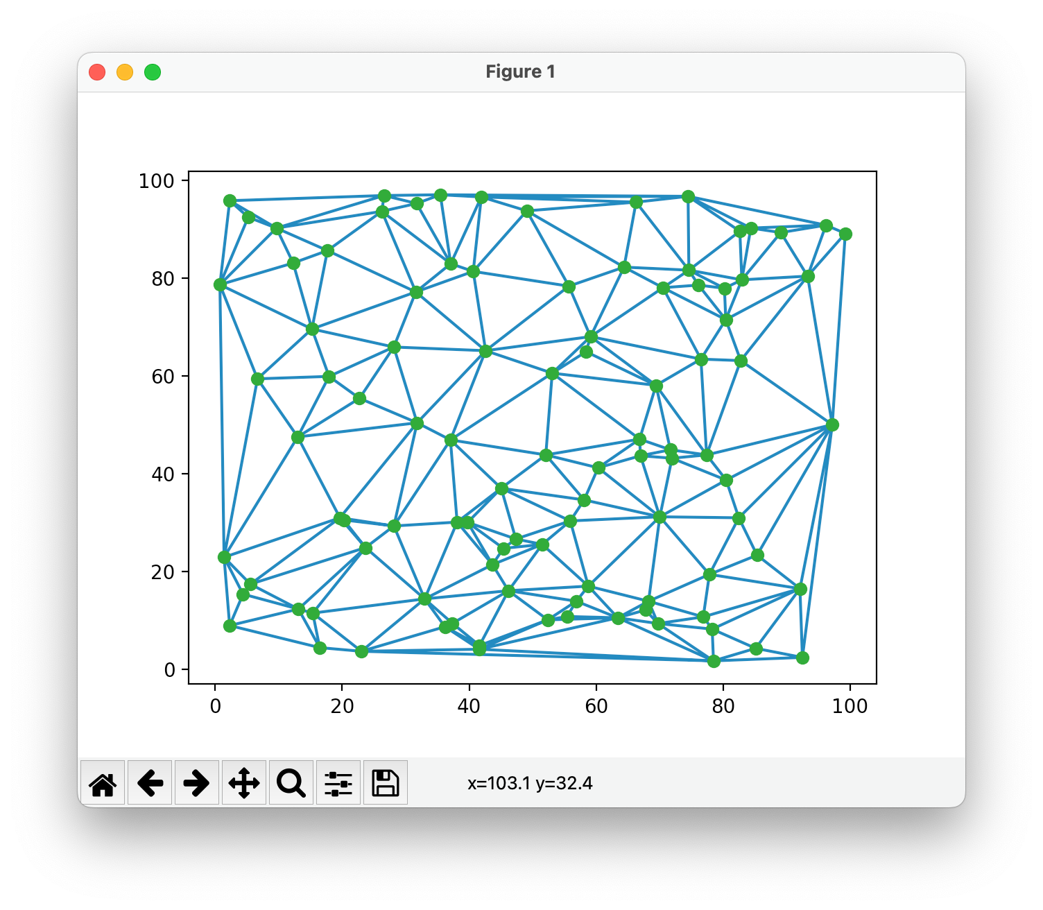
Plotting the DT with matplotlib
import startinpy
import numpy as np

#-- generate 100 points randomly in the plane
rng = np.random.default_rng(seed=42)
pts = rng.random((100, 3))
#-- scale to [0, 100]
pts = pts * 100
t = startinpy.DT()
t.insert(pts)
pts = t.points
trs = t.triangles
#-- plot
import matplotlib.pyplot as plt
plt.triplot(pts[:,0], pts[:,1], trs)
#-- the vertex "0" shouldn't be plotted, so start at 1
plt.plot(pts[1:,0], pts[1:,1], 'o')
plt.show()
Gridding the dataset with spatial interpolation
import startinpy
import numpy as np
import json
import laspy
import rasterio
import math
from tqdm import tqdm

def main():
    las = laspy.read("../data/small.laz")
    dt = startinpy.DT()
    dt.duplicates_handling = "Highest"
    d = las.xyz
    print("Constructing the TIN with {} points".format(len(d)))
    for each in tqdm(d):
        dt.insert_one_pt(each)

    #-- grid with 50cm resolution the bbox
    bbox = dt.get_bbox()
    cellsize = 0.5
    deltax = math.ceil((bbox[2] - bbox[0]) / cellsize)
    deltay = math.ceil((bbox[3] - bbox[1]) / cellsize)
    centres = []
    i = 0
    for row in range((deltay - 1), -1, -1):
        j = 0
        y = bbox[1] + (row * cellsize) + (cellsize / 2)
        for col in range(deltax):
            x = bbox[0] + (col * cellsize) + (cellsize / 2)
            centres.append([x, y])
            j += 1
        i += 1
    centres = np.asarray(centres)
    print("Interpolating at {} locations".format(centres.shape[0]))
    zhat = dt.interpolate({"method": "TIN"}, centres)
    # zhat = dt.interpolate({"method": "Laplace"}, centres)
    # zhat = dt.interpolate({"method": "IDW", "radius": 20, "power": 2.0}, centres, strict=True)

    #-- save to a GeoTIFF with rasterio
    write_rasterio('grid.tiff', zhat.reshape((deltay, deltax)), (bbox[0], bbox[1]), cellsize)

def write_rasterio(output_file, a, bbox, cellsize):
    with rasterio.open(output_file, 'w',
                       driver='GTiff',
                       height=a.shape[0],
                       width=a.shape[1],
                       count=1,
                       dtype=np.float32,
                       crs=rasterio.crs.CRS.from_string("EPSG:28992"),
                       nodata=np.nan,
                       transform=(cellsize, 0., bbox[1], 0., -cellsize, bbox[0])) as dst:
        dst.write(a, 1)
    print("File written to '%s'" % output_file)

if __name__ == '__main__':
    main()